

Empowering Developers for Seamless Collaboration with GitHub Tools

Empowering Developers for Seamless Collaboration with GitHub Tools

GitHub has evolved from a Git hosting service into a comprehensive developer platform offering issue tracking, CI/CD (GitHub Actions), package registry, code scanning, project management, and wiki documentation. These integrated tools streamline the entire software development lifecycle within a single interface, reducing context switching and enabling seamless collaboration for distributed teams.

GitHub Issues and Project Management

GitHub Issues track bugs, feature requests, and tasks with labels, assignees, milestones, and linked pull requests. The modern issue experience includes issue templates (standardized formats for bug reports and feature requests), issue forms (structured YAML-defined forms with validation), and task lists within issues for tracking sub-tasks. GitHub Projects provides a Kanban-style board that automatically syncs with issues and PRs, supporting custom workflows with status fields, iterations, and insights dashboards. Automations can move cards between columns based on label changes, PR merges, or scheduled dates, reducing manual board management.

# Using GitHub CLI to manage issues
gh issue create --title "Add dark mode" --body "Users have requested a dark theme..."   --label enhancement --assignee @me --project "Q3 Sprint"

gh issue list --label bug --assignee @me
gh issue view 42  # View issue details in terminal

# Link PR to issue automatically (mention in PR description)
# Closes #42 — PR will auto-close the issue when merged

GitHub Actions for CI/CD

GitHub Actions provides workflow automation triggered by GitHub events (push, PR, schedule, issue creation). Workflows are YAML files in .github/workflows/ that define jobs running on GitHub-hosted or self-hosted runners. Each job consists of steps that can run commands or use pre-built actions from the Marketplace. Common workflows include running tests on every push, deploying to cloud platforms on merge to main, publishing packages to npm or Docker Hub on version tags, and scheduled tasks like dependency updates or database backups.

# .github/workflows/ci.yml
name: CI
on: [push, pull_request]
jobs:
  test:
    runs-on: ubuntu-latest
    steps:
      - uses: actions/checkout@v4
      - uses: actions/setup-python@v5
        with: { python-version: "3.12" }
      - run: pip install -r requirements.txt
      - run: pytest --cov=src --cov-report=xml
      - uses: codecov/codecov-action@v4
  deploy:
    needs: test
    if: github.ref == 'refs/heads/main'
    runs-on: ubuntu-latest
    steps:
      - uses: actions/checkout@v4
      - uses: superfly/flyctl-actions@1.5
        with: { args: "deploy" }
        env: { FLY_API_TOKEN: ${{ secrets.FLY_API_TOKEN }} }

Code Review with Pull Requests

GitHub’s pull request interface supports inline code comments, suggested changes (one-click accept), draft PRs (mark work-in-progress without triggering CI), and required reviewers with branch protection rules. Review assignment can be automatic (code owners file, load balancing round-robin). Conversation resolution tracks when comments are addressed. The Checks tab shows CI status directly in the PR. Merge queues (GitHub Merge Queue) automatically test PRs in batches before merging, ensuring main is always green even with concurrent merges. For security-sensitive projects, CODEOWNERS can enforce that specific files require review from designated teams.

Security Features

Dependabot automatically scans dependencies for known vulnerabilities (from GitHub Advisory Database) and creates PRs to update them. Secret scanning detects exposed credentials (API keys, tokens, passwords) in repositories and alerts the security team. CodeQL analysis runs static analysis on every push, finding security vulnerabilities (SQL injection, XSS, path traversal) and code quality issues. SBOM (Software Bill of Materials) generation outputs a machine-readable inventory of all dependencies, helping with supply chain security compliance. These security features, combined with mandatory 2FA enforcement and SAML/SSO for organizations, make GitHub a secure platform for enterprise development teams.

GitHub Actions Advanced Patterns

GitHub Actions supports matrices (running the same job with different OS or language versions), reusable workflows (calling a workflow from another workflow, avoiding duplication), environments (with approval gates and secrets scoped to deployment targets), and composite actions (bundling multiple steps into a reusable action). For monorepos, paths filtering triggers workflows only when specific directories change. The concurrency group prevents duplicate workflow runs on the same branch. Workflow commands allow creating annotations, setting outputs, and updating the job summary from within script steps. Artifact and cache actions speed up builds by persisting dependencies between runs. For self-hosted runners, autoscaling with actions-runner-controller on Kubernetes provides enterprise-level capacity management.

# Matrix testing across Python versions and OS
jobs:
  test:
    strategy:
      matrix:
        os: [ubuntu-latest, macos-latest, windows-latest]
        python: ["3.9", "3.10", "3.11", "3.12"]
    runs-on: ${{ matrix.os }}
    steps:
      - uses: actions/setup-python@v5
        with: { python-version: ${{ matrix.python }} }
      - run: pip install . && pytest

GitHub Pages and Documentation

GitHub Pages hosts static websites directly from repositories, supporting Jekyll, Hugo, and plain HTML. Project pages (served from a gh-pages branch or /docs folder) provide free documentation hosting with custom domain support and automatic HTTPS. Pages integrates with Actions: build your static site generator, deploy the output to Pages, and invalidate the CDN cache automatically. GitHub Wikis provide collaborative documentation that anyone with repository access can edit, with version history and search. For API documentation, GitHub’s support for OpenAPI/Swagger renders specification files directly in the repository view. Combined with the GitHub REST API and GraphQL API, you can automate documentation generation and maintain a project website without leaving the GitHub ecosystem.
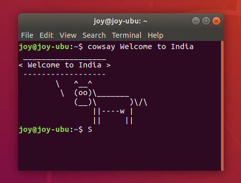
Mastering the Command Line Interface (CLI): Exploring Bash, Terminal, Command Prompt & PowerShell

CLI stands for Command Line Interface, which is a way of interacting with a computer program or operating system through a text-based interface rather than a graphical user interface (GUI). A CLI allows users to enter commands into a command prompt or terminal window to perform tasks such as navigating the file system, running programs, and configuring system settings.

Bash, Terminal, Command Prompt, and Power Shell are all examples of command-line interfaces used in different operating systems.

Bash (Bourne-Again SHell) is a popular shell program that is commonly used on Linux and other Unix-based operating systems. It provides a command-line interface for executing commands, running scripts, and manipulating files and directories. Some useful features of Bash are:

  1. Scripting Capabilities: Bash is a powerful scripting language that allows for automation and the creation of complex scripts and programs.
  2. Availability: Bash is pre-installed on most Linux and Unix-based systems, making it readily available for use.
  3. Customizability: Bash can be customized to meet the needs of the user with the use of scripts, aliases, and configuration files.
  4. Interoperability: Bash can work with a wide range of command-line tools and utilities, making it compatible with many different systems and applications.
  5. Flexibility: Bash can be used for a variety of tasks, from simple one-liner commands to complex shell scripts.

Bash is a powerful and flexible command-line interface and scripting language, but its complexity and limitations may make it challenging for some users. Some of these challenges are:

  1. Steep Learning Curve: Bash can be difficult to learn for beginners, due to its syntax and many different commands and utilities.
  2. Limited Graphical Capabilities: Bash is primarily a command-line interface and does not have strong graphical capabilities, which can be limiting for certain tasks.
  3. Security Risks: Bash scripts and commands can potentially introduce security risks if not properly written or managed.
  4. Platform Dependence: While Bash is available on most Linux and Unix-based systems, it may not be available on other operating systems, which can limit its portability.
  5. Limited Interactivity: Bash is primarily used for running commands and scripts and may not be as interactive or user-friendly as other interfaces for certain tasks.

Terminal is a command-line interface that is used on Apple’s macOS operating system. It provides a window where users can enter commands and interact with the operating system. In many Linux distros CLI application has the name ‘Terminal’. While the names of the terminal applications may be the same on Linux and MacOS, there are differences in the way they function as underlying operating systems are not same. Linux terminal is usually Bash, while the default shell used in the macOS terminal is Zsh. Many of the command-line tools and utilities available in the Linux terminal are also available in the macOS terminal, there may be some differences in the versions or implementations of these tools

Command Prompt is a command-line interface that is used on Microsoft Windows operating systems. It provides a window where users can enter commands to perform tasks such as navigating the file system, running programs, and configuring system settings.

Power Shell is also a command-line interface developed by Microsoft for modern Windows operating systems. It provides an extensive scripting language and can be used to automate administrative tasks and system configuration.

While Cmd(Command Prompt) and PowerShell are both command-line interfaces used in Windows operating systems. There are some key differences between the two:

  1. Functionality: PowerShell is more powerful and feature-rich than Cmd, with support for advanced scripting and automation tasks. PowerShell also has access to .NET Framework libraries, allowing for more advanced scripting capabilities.
  2. Syntax: PowerShell uses a different syntax than Cmd, using cmdlets (short for “command-lets”) instead of traditional commands. Cmdlets are structured in a verb-noun format, making it easier to remember and use them.
  3. Command Support: PowerShell supports most of the commands available in Cmd, but also has its own set of unique commands. Cmd does not have access to many of the advanced features available in PowerShell.
  4. Output Formatting: PowerShell has more flexible output formatting options, allowing users to easily customize and filter output data. Cmd has limited output formatting capabilities.
  5. Cross-Platform Support: PowerShell is cross-platform, with versions available for Windows, Linux, and macOS. Cmd is only available on Windows operating systems.
  6. Learning Curve: PowerShell has a steeper learning curve than Cmd, due to its more complex syntax and advanced features.

While these CLI tools have different names and are used on different operating systems, they all provide similar functionality in terms of allowing users to enter commands to interact with the operating system and perform various tasks.

An interesting practical example to see the similarity and differences between these popular CLIs is the command to change the encoding of a file to ‘UTF-8’.

In Bash (on Linux or Unix-based systems) the command is iconv and has following syntax:

iconv -f [source_encoding] -t UTF-8 [input_file] > [output_file]

For example, to convert a file encoded in ISO-8859-1 to UTF-8 using Bash:

iconv -f ISO-8859-1 -t UTF-8 input.txt > output.txt

In Terminal (on macOS) the name of command is same but syntax is slightly different:

iconv -f [source_encoding] -t UTF-8 -o [output_file] [input_file]

For example, to convert a file encoded in ISO-8859-1 to UTF-8 using MacOS Terminal:

iconv -f ISO-8859-1 -t UTF-8 -o output.txt input.txt

On Command Prompt (on Windows) the command is ‘chcp’ and its syntax is:

chcp [code_page_number] & type [input_file] > [output_file]

For example, to convert a file encoded in ANSI (Windows-1252) to UTF-8 the command is:

chcp 1252 & type input.txt > output.txt

Power Shell (on Windows):

Get-Content -Path [input_file] -Encoding [source_encoding] | Set-Content -Path [output_file] -Encoding UTF8

For example, to convert a file encoded in ANSI (Windows-1252) to UTF-8 in Power Shell the command is:

Get-Content -Path input.txt -Encoding Default | Set-Content -Path output.txt -Encoding UTF8

Shell Scripting and Automation

The command line is the most productive interface for system administration, development workflows, and data processing. Essential commands include: ls (list files), find (search files by name/type/size), grep (search content), awk (text processing), sed (stream editing), chmod (permissions), ps (process status), top/htop (resource monitoring), and ssh (remote access). Combining commands with pipes (|) creates powerful one-liners: ps aux | grep python lists Python processes; find . -name “*.py” | xargs wc -l counts lines in all Python files. Shell scripts (.sh files) automate repetitive tasks with variables, conditionals, loops, and functions. Learn to use tab completion, command history (Ctrl+R for reverse search), and job control (Ctrl+Z to suspend, fg/bg to resume). The command line is not optional for professional developers—every deployment, debugging session, and data pipeline relies on CLI proficiency.

# One-liner to find largest files
find /var/log -type f -size +100M -exec ls -lh {} \; | sort -k5 -hr

# Count unique IPs in access log
awk '{print $1}' /var/log/nginx/access.log | sort | uniq -c | sort -rn | head -10

Generating a Date Column from Month, Day, and Year in Python Pandas

Generating a Date Column from Month, Day, and Year in Python Pandas

When working with real-world datasets, dates are often split across multiple columns—month, day, and year stored separately. Combining them into a proper datetime column enables time-based filtering, resampling, date arithmetic, and plotting. Python’s Pandas library provides several approaches, each suited to different data formats and performance requirements.

Using pd.to_datetime with a Dictionary

The most readable approach passes a dictionary mapping column names to date parts. Pandas’s to_datetime function accepts year, month, day keys and assembles them into datetime objects. This works directly on DataFrame columns without looping or apply functions. Missing or invalid dates (like February 30) produce NaT (Not a Time) values by default, which you can then handle with fillna or dropna.

import pandas as pd

df = pd.DataFrame({
    "year": [2024, 2024, 2024, 2024],
    "month": [1, 2, 3, 2],
    "day": [15, 28, 1, 30]
})

df["date"] = pd.to_datetime(df[["year", "month", "day"]])
print(df)
#    year  month  day       date
# 0  2024      1   15 2024-01-15
# 1  2024      2   28 2024-02-28
# 2  2024      3    1 2024-03-01
# 3  2024      2   30 2024-02-30  # NaT (invalid date)

# Drop invalid dates
df = df.dropna(subset=["date"])

String Concatenation Approach

An alternative method concatenates the columns into a date string and parses it. This is useful when you have additional columns like hour, minute, second, or timezone that you want to include. The f-string or .str.cat() approach creates a standard ISO format string (YYYY-MM-DD) that to_datetime parses efficiently. For large datasets (millions of rows), the dictionary method is faster because it avoids string creation overhead, but the string method offers more flexibility for non-standard date formats.

# String concatenation method
df["date_str"] = (df["year"].astype(str) + "-" +
                  df["month"].astype(str).str.zfill(2) + "-" +
                  df["day"].astype(str).str.zfill(2))
df["date"] = pd.to_datetime(df["date_str"])

# More concise: using assign and f-string
df = df.assign(date=pd.to_datetime(
    df["year"].astype(str) + "-" +
    df["month"].astype(str).str.zfill(2) + "-" +
    df["day"].astype(str).str.zfill(2)
))

Handling Different Column Names

Real datasets use varying column names. The dictionary approach handles this by renaming on the fly: pd.to_datetime(df[[“yr”, “mo”, “dy”]].rename(columns={“yr”:”year”,”mo”:”month”,”dy”:”day”})). For datasets with century prefixes (e.g., year column has values 23 instead of 2023), add 2000 before conversion. When month or day names are used instead of numbers (“January” instead of 1), use pd.to_datetime(df[“month”], format=”%B”) first to convert month names to numbers before combining.

# Rename columns to match expected names
cols = {"yr": "year", "mon": "month", "d": "day"}
df["date"] = pd.to_datetime(df[["yr", "mon", "d"]].rename(columns=cols))

# Handle 2-digit years
df["full_year"] = df["yr"] + 2000
df["date"] = pd.to_datetime(df[["full_year", "month", "day"]])

# For month names instead of numbers
df["month_num"] = pd.to_datetime(df["month_name"], format="%B").month

Performance Considerations

For small datasets (under 100K rows), all methods are fast enough. For millions of rows, the dictionary method (pd.to_datetime(df[[cols]])) is the fastest because it operates on integer columns directly without string conversion. Adding parsed dates as a DatetimeIndex enables efficient resampling (.resample()), time-based slicing (.loc[“2024-01″:]), and date-based aggregations (.groupby(pd.Grouper(freq=”ME”))). Once your data has a proper datetime column, you unlock the full Pandas time series toolkit—rolling windows, shifting, differencing, and timezone-aware operations.

Working with Time Series After Date Creation

Once you have a proper datetime column, set it as the DataFrame index with df.set_index(‘date’). This enables powerful time series operations: df.resample(‘M’).mean() computes monthly averages, df[‘2024′] selects all data from 2024, and df.rolling(7).mean() computes a 7-day moving average. For financial data, you can compute day-over-day changes with .diff(), year-over-year comparisons with .pct_change(periods=365), and cumulative sums with .cumsum(). Timezone-aware datetime columns (use tz=’UTC’ or tz=’Asia/Kolkata’ in to_datetime) handle daylight saving transitions correctly. Pandas also supports custom business calendars (pd.offsets.CustomBusinessDay) for financial data that excludes holidays and weekends. These operations form the foundation of time series analysis in Python, used across finance, IoT sensor data, web analytics, and scientific research.

df['date'] = pd.to_datetime(df[['year','month','day']])
df = df.set_index('date')
monthly = df.resample('ME').mean()  # Month-end frequency
weekly_rolling = df['value'].rolling(7, center=True).mean()
df['pct_change'] = df['value'].pct_change()

Handling Missing Date Components

Real datasets often have missing day or month values. If only year and month are known, set day to 1 as a convention. If month is missing but quarter is available, map quarter (Q1=month 1, Q2=4, Q3=7, Q4=10). The nullable integer type (pd.Int32Dtype()) allows integer columns to hold NA values that to_datetime can propagate as NaT. For datasets where dates span centuries (birth years from 1920-2020), ensure 2-digit years are parsed correctly by specifying the century cutoff with pd.to_datetime(col, format=’%m/%d/%y’, errors=’coerce’). Always validate the resulting dates by checking range: dates in the future or before the dataset’s expected timeframe indicate parsing errors. Visualizing the date distribution with df[‘date’].hist() quickly reveals outliers and gaps in the temporal coverage of your data.

Complex Numbers: The Argand Plane and Euler’s Formula

Complex Numbers: The Argand Plane and Euler’s Formula

Complex numbers extend the real number system by including the imaginary unit i, where i² = -1. Every complex number is written as z = a + bi, where a is the real part and b is the imaginary part. The Argand plane (complex plane) visualizes complex numbers as points with real coordinates (a, b). Euler’s formula, e^(iθ) = cos θ + i sin θ, connects exponential functions to trigonometry and is fundamental to electrical engineering, quantum mechanics, signal processing, and control theory.

The Argand Plane

The Argand plane is a 2D coordinate system where the x-axis represents the real part and the y-axis represents the imaginary part. The complex number 3 + 4i becomes the point (3, 4). The distance from the origin to the point is the modulus (or magnitude): |z| = √(a² + b²). The angle from the positive real axis is the argument (or phase): arg(z) = arctan(b/a). This geometric interpretation makes operations intuitive: addition is vector addition, multiplication combines moduli and adds arguments (|z₁z₂| = |z₁||z₂|, arg(z₁z₂) = arg(z₁) + arg(z₂)).

import cmath, math

# Complex numbers in Python
z1 = 3 + 4j
z2 = 1 - 2j

# Basic operations
print(f"z1 = {z1}, |z1| = {abs(z1):.2f}, arg(z1) = {cmath.phase(z1):.3f} rad")
print(f"z2 = {z2}, |z2| = {abs(z2):.2f}")
print(f"z1 + z2 = {z1 + z2}")
print(f"z1 * z2 = {z1 * z2}")
print(f"|z1 * z2| = {abs(z1 * z2):.2f}")  # = |z1| * |z2|

Euler’s Formula and Polar Form

Euler’s formula e^(iθ) = cos θ + i sin θ is the most important equation in complex analysis. It allows representing complex numbers in polar form: z = re^(iθ) where r = |z| and θ = arg(z). This form makes multiplication, division, and exponentiation trivial: multiply by multiplying radii and adding angles; raise to a power by raising the radius and multiplying the angle (De Moivre’s theorem). The special case e^(iπ) + 1 = 0 (Euler’s identity) connects five fundamental mathematical constants in a single equation.

# Polar form and Euler's formula
theta = math.pi / 4  # 45 degrees
z_polar = cmath.rect(1.0, theta)  # cos(π/4) + i·sin(π/4)
print(f"e^(iπ/4) = {z_polar:.3f}")
print(f"cos(π/4) = {math.cos(theta):.3f}, sin(π/4) = {math.sin(theta):.3f}")

# De Moivre's theorem: (cos θ + i sin θ)^n = cos(nθ) + i sin(nθ)
z = cmath.rect(1, math.pi/6)  # e^(iπ/6)
z_cubed = z ** 3
expected = cmath.rect(1, math.pi/2)  # e^(iπ/2) = i
print(f"(e^(iπ/6))³ = {z_cubed:.3f}, expected {expected:.3f}")

Applications in Signal Processing

The Fast Fourier Transform (FFT), implemented in NumPy as np.fft.fft(), decomposes signals into their frequency components using complex exponentials. Each frequency component is a complex number: the magnitude represents amplitude, and the argument represents phase. This is essential for audio processing (equalizers, compression), image processing (JPEG uses a related transform), wireless communications (OFDM), and control systems (frequency response analysis). In electrical engineering, complex impedance (Z = R + jX) replaces resistance for AC circuits, with the imaginary part representing reactance from capacitors and inductors.

import numpy as np
import matplotlib.pyplot as plt

# FFT of a signal with two frequencies
fs = 1000  # Sampling rate
t = np.linspace(0, 1, fs, endpoint=False)
signal = np.sin(2 * np.pi * 50 * t) + 0.5 * np.sin(2 * np.pi * 120 * t)

fft = np.fft.fft(signal)
freqs = np.fft.fftfreq(fs, 1/fs)
magnitude = np.abs(fft[:fs//2])  # Magnitude spectrum

# Peaks at 50 Hz and 120 Hz confirm signal composition
peak_freqs = freqs[:fs//2][magnitude > 100]
print(f"Detected frequencies: {peak_freqs} Hz")
# Phase information (from complex argument) gives timing/alignment

Complex numbers are also fundamental to quantum mechanics (wave functions are complex-valued, and the Schrödinger equation uses i∂ψ/∂t), fluid dynamics (potential flow theory uses complex potentials), and fractal generation (the Mandelbrot set is defined by iterating z ← z² + c in the complex plane). Python’s built-in complex type and the cmath, numpy, and scipy libraries provide comprehensive support for complex arithmetic, making it practical to work with complex numbers in any computational domain.

Complex Numbers in Python and NumPy

Python provides first-class support for complex numbers with the j suffix (3+4j) and the complex() constructor. The cmath module mirrors math but for complex arguments: cmath.sqrt(-1) returns 1j, while math.sqrt(-1) raises ValueError. NumPy extends this to array operations: np.array([1+2j, 3+4j]) creates a complex array, and ufuncs like np.sin, np.exp, and np.sqrt work natively on complex arrays. NumPy’s FFT functions return complex arrays where the real part represents cosine amplitudes and the imaginary part represents sine amplitudes. For scientific computing, complex numbers enable solving differential equations (the Schrödinger equation uses i∂ψ/∂t), representing AC circuits (impedance Z = R + jX), and computing the Mandelbrot set (iterating z = z² + c on the complex plane). The matplotlib library plots complex functions using domain coloring, where hue represents argument and brightness represents magnitude, providing a complete visualization of complex-valued functions in a single image.

Complex Numbers in Python and NumPy

Python provides first-class support for complex numbers with the j suffix (3+4j) and the complex() constructor. The cmath module mirrors math but for complex arguments: cmath.sqrt(-1) returns 1j, while math.sqrt(-1) raises ValueError. NumPy extends this to array operations: np.array([1+2j, 3+4j]) creates a complex array, and ufuncs like np.sin, np.exp, and np.sqrt work natively on complex arrays. NumPy’s FFT functions return complex arrays where the real part represents cosine amplitudes and the imaginary part represents sine amplitudes. For scientific computing, complex numbers enable solving differential equations, representing AC circuits (impedance Z = R + jX), and computing the Mandelbrot set (iterating z = z^2 + c on the complex plane).

Python Program to Print Powers from 1 to 5 of Numbers from 1 to 20

Python Program to Print Powers from 1 to 5 of Numbers from 1 to 20

Computing powers of numbers is a fundamental programming exercise that demonstrates loops, formatting, and mathematical operations in Python. This article explores multiple approaches to printing the powers (x^1 through x^5) for numbers 1 through 20, ranging from basic loops to NumPy-based vectorized solutions. Each approach teaches different Python concepts while producing the same tabular output.

Basic Nested Loop Approach

The simplest solution uses two nested for loops: an outer loop iterating numbers 1 through 20, and an inner loop computing powers 1 through 5. Python’s exponentiation operator (**) computes powers efficiently. Using formatted string literals (f-strings) with width specifiers aligns the output into readable columns. The print() function’s end parameter controls spacing between columns, and an empty print() at the end of each row creates the line break.

# Print powers 1-5 for numbers 1-20
for num in range(1, 21):
    for exp in range(1, 6):
        result = num ** exp
        print(f"{result:>10}", end=" ")
    print()  # New line after each row

Using List Comprehension for Compact Code

List comprehensions generate each row as a list of power values, then join them into a formatted string. This approach is more Pythonic and separates data generation from presentation. The join() method with formatted strings avoids repeated print() calls, which is slightly more performant for large outputs. The pattern also teaches an important skill: separating computation logic from output formatting, making the code easier to modify or repurpose.

for num in range(1, 21):
    row = [str(num ** exp).rjust(10) for exp in range(1, 6)]
    print(" ".join(row))

NumPy Vectorized Solution

For maximum performance (especially with larger ranges), NumPy’s broadcasting computes all powers at once. The outer product of two arrays—numbers and exponents—creates a 2D matrix where element (i,j) = numbers[i]^exponents[j]. NumPy’s vectorized operations execute in C, making this approach orders of magnitude faster for large ranges. This introduces the concept of broadcasting, one of NumPy’s most powerful features for eliminating explicit Python loops.

import numpy as np

numbers = np.arange(1, 21).reshape(-1, 1)  # Column vector (20,1)
exponents = np.arange(1, 6)                # Row vector    (1,5)
powers = numbers ** exponents              # Broadcast →  (20,5)

# Format and print
for row in powers:
    print(" ".join(f"{val:>10}" for val in row))

Understanding the Output Pattern

The output is a 20×5 matrix where each row shows increasing powers of a number: row 1 is 1^1=1, 1^2=1, 1^3=1, 1^4=1, 1^5=1; row 10 is 10, 100, 1000, 10000, 100000; and row 20 grows exponentially to 20, 400, 8000, 160000, 3200000. This exercise teaches iteration, exponentiation, formatted output, and the relationship between numbers and their powers. The same pattern extends to other mathematical functions like factorials, Fibonacci sequences, or multiplication tables, reinforcing the general concept of nested iteration over parameter ranges.

Extending the Program with User Input

Making the program interactive with user-specified ranges makes it more flexible. Using input() and sys.argv, users can set the maximum number, the exponent range, and output format (table vs CSV). Adding file output with redirect (python powers.py > output.txt) or programmatic CSV generation makes the data usable in spreadsheet applications. Error handling for non-numeric input and unreasonably large ranges (where numbers overflow Python’s arbitrary-precision integers) prevents crashes. Python’s integers have arbitrary precision, so 20^5 = 3.2 million prints correctly, but 100^100 has 201 digits and prints without overflow—something many languages cannot do. This exercise also demonstrates the computational cost: computing powers for numbers up to 10,000 with exponents to 10 generates 100,000 calculations, showcasing the difference between O(n) and O(n×m) complexity.

import sys
max_num = int(sys.argv[1]) if len(sys.argv) > 1 else 20
max_exp = int(sys.argv[2]) if len(sys.argv) > 2 else 5
import csv, io
output = io.StringIO()
writer = csv.writer(output)
writer.writerow(['number'] + [f'^{e}' for e in range(1, max_exp+1)])
for n in range(1, max_num+1):
    writer.writerow([n] + [n**e for e in range(1, max_exp+1)])
print(output.getvalue())

Mathematical Patterns in Power Sequences

Computing power sequences reveals interesting mathematical patterns. Numbers ending in 0 always end in 0 for any exponent. Numbers ending in 1, 5, or 6 always end in the same digit (1^5 ends in 1, 6^3 ends in 6). Numbers ending in 2 cycle through 2, 4, 8, 6. Numbers ending in 3 cycle through 3, 9, 7, 1. These patterns come from modular arithmetic: the last digit of a power depends only on the last digit of the base, and the cycle length divides 4 (by Euler’s theorem). The sequence 1^n = 1 for all n, while 2^10 = 1024 grows past 1000. This exercise demonstrates exponential growth, modulo arithmetic, and the difference between polynomial and exponential functions—concepts foundational to algorithm analysis and computational complexity theory.